Video to Point Cloud Art

I like crabs (you might have noticed). Also, the home page was still a bit boring without any background. That’s why I was looking for something that’s visually interesting, but not too colorful.

Generating the depth

#

The idea is to create a monochromatic 3D point-cloud visualization of a crab that explores glitchy, cyber-retro visual aesthetics.

Then I remembered that I had been playing around with an XBOX Kinect v2 sensor, using its depth data to create abstract visualizations in Blender. What if I could do that, but with crabs? I briefly considered building an underwater case for the Kinect, which has already been done in this paper. But I quickly realized that this would be quite a task, as I’d need to carry a battery and a small PC underwater as well.

Alternatively, I could make a small swimming buoy and run only a cable to the sensor underwater. However, that still sounded quite complicated. The next idea was to use two GoPros on a small rig, essentially forming an underwater stereo setup. But that would require careful calibration as well as synchronization between the two sensors.

Then I finally got the idea to use monocular depth estimation to estimate depth from my images. While this technology isn’t at a point where I’d trust a vehicle to use it as a single source of truth for self driving, it’s good enough for what I want to do.

The initial test using Intel DPT

#

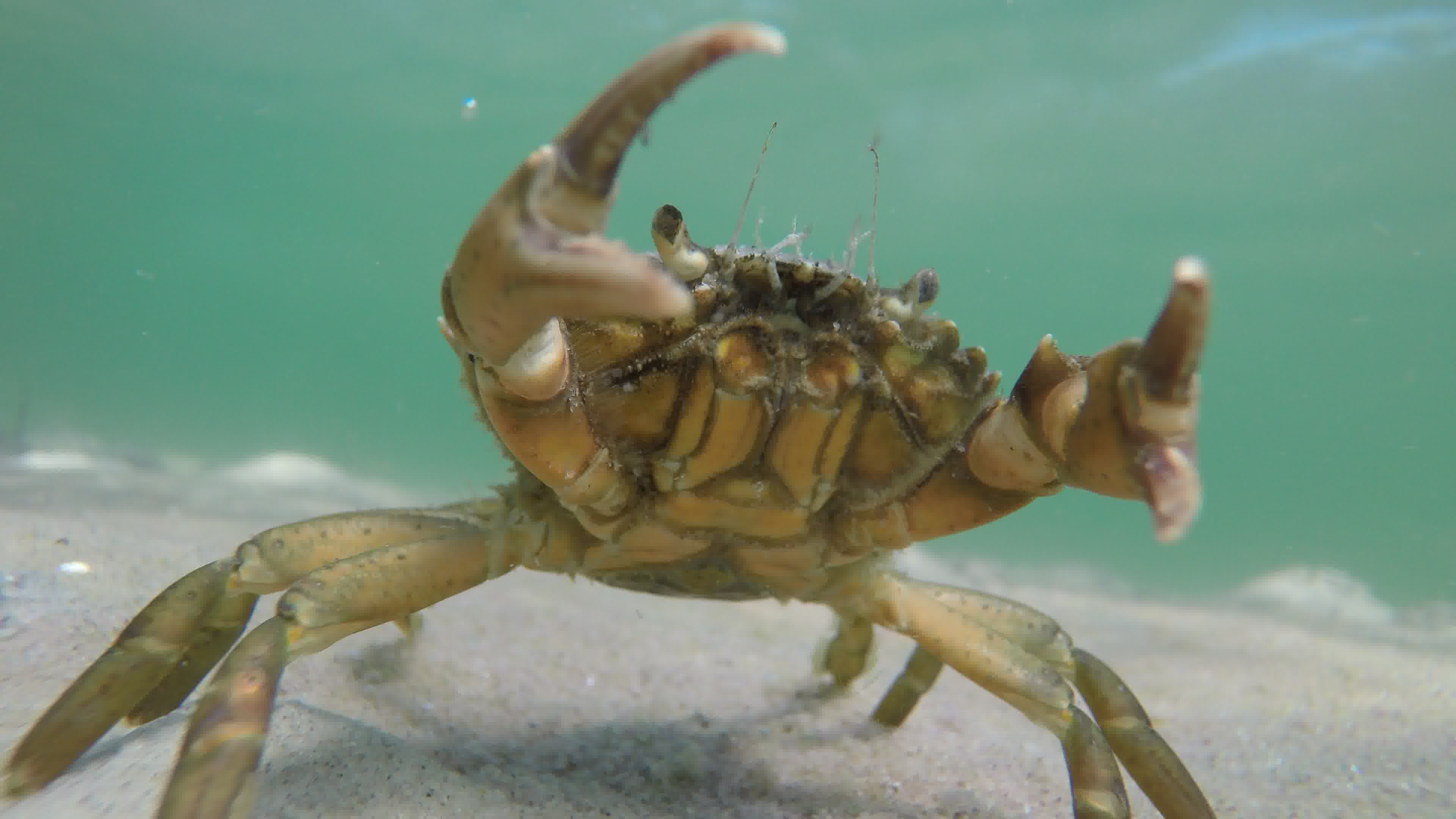
So I started by looking through the videos from my last scuba diving adventure in the Baltic Sea, and I came across a video of a close up crab:

I then looked online for some easy-to-use local depth estimation models and came across the DPT-large from Intel on huggingface. The model ran on my 12th-gen i5 Framework laptop at about one frame every two seconds. However, the results I was seeing were meh.

To use this model, I needed to convert the video sequence into an image sequence and then run depth estimation on every frame. I did that using ffmpeg via ffmpeg -i input.mp4 out%d.png. This might already ring a bell if you’re familiar with neural network image processing: since the output is essentially black-box guesswork, and each frame has no information about the previous one, there’s no depth-wise continuity at all between consecutive frames.

I ran the images through the network by basically looping over the minimal working example from the huggingface page for every generated png and storing the depth directly into a sequence of ply files. This way I was able to easily import the data in blender.

def main():
    # Set up environment
    input_dir = Path("data/video1/images/")
    output_dir = Path("data/video1/depths/")
    estimator = pipeline(task="depth-estimation",
                         model="Intel/dpt-large")

    # Get list of files in input folder
    image_files = [p for p in input_dir.glob("*") if p.suffix.lower() in [".jpg", ".png"]]

    for img_path in image_files:
        print("Processing:", img_path.name)

        # Load
        img = cv2.imread(str(img_path))
        img_rgb = cv2.cvtColor(img, cv2.COLOR_BGR2RGB)

        # Convert to PIL
        img_pil = Image.fromarray(img_rgb)

        # Inference
        result = estimator(img_pil)
        depth = np.array(result["depth"]).astype(np.float32)

        # Output path
        ply_path = output_dir / (img_path.stem + ".ply")

        # Save as PLY
        save_depth_as_ply(depth, img_rgb, ply_path)

    print("Done! PLY files saved to:", output_dir)

if __name__ == "__main__":
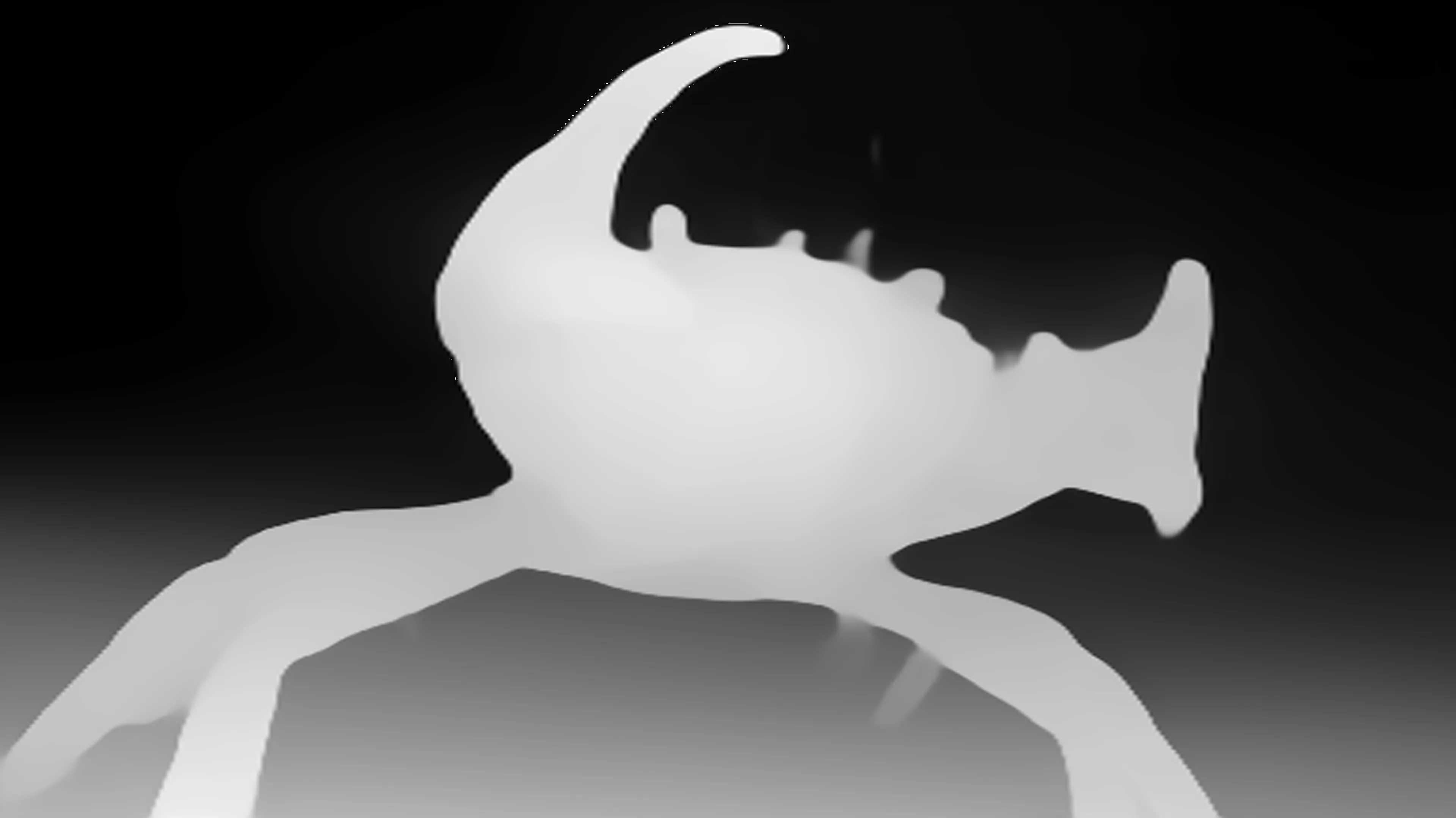
    main()

Another interesting observation was that the orientation of the image matters. Again, this isn’t a surprise if you consider that the network was most likely trained only on right-side-up imagery. The GoPro filming the footage was mounted to a long pole, and to get close to the sand I had to hang the camera upside down. So I naively tried feeding the flipped images into the DPT model — and the results were very, very soft. When flipping over the image \(180^\circ\), the output becomes much more crisp.

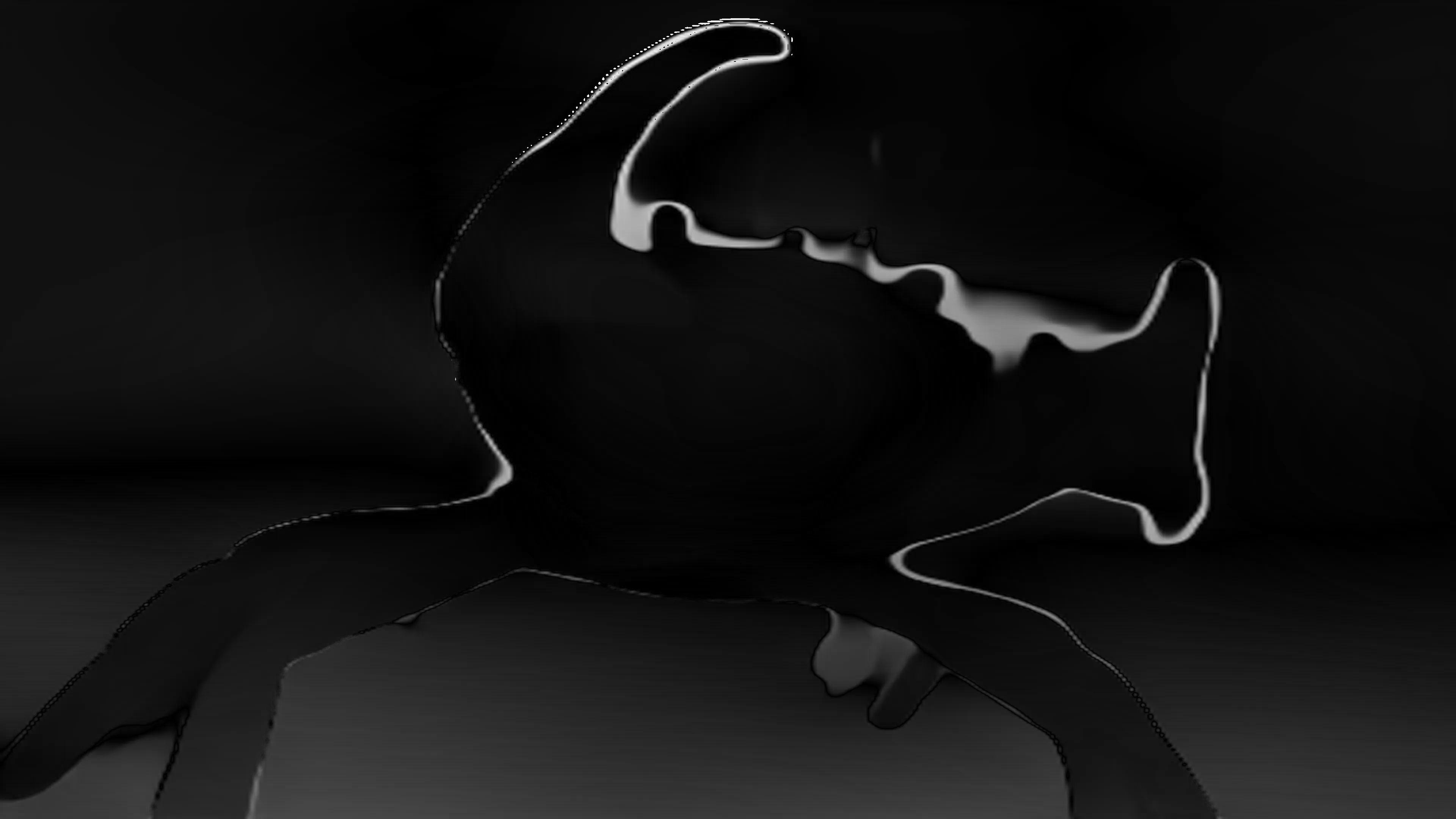
The depth estimation for the rotated image looks much better than the previous one. The eye and claw section looks much more defined now, which is confirmed by the difference image. While the depth images look better now, we can look at the point cloud in CloudCompare to see if the result still looks plausible in that domain.

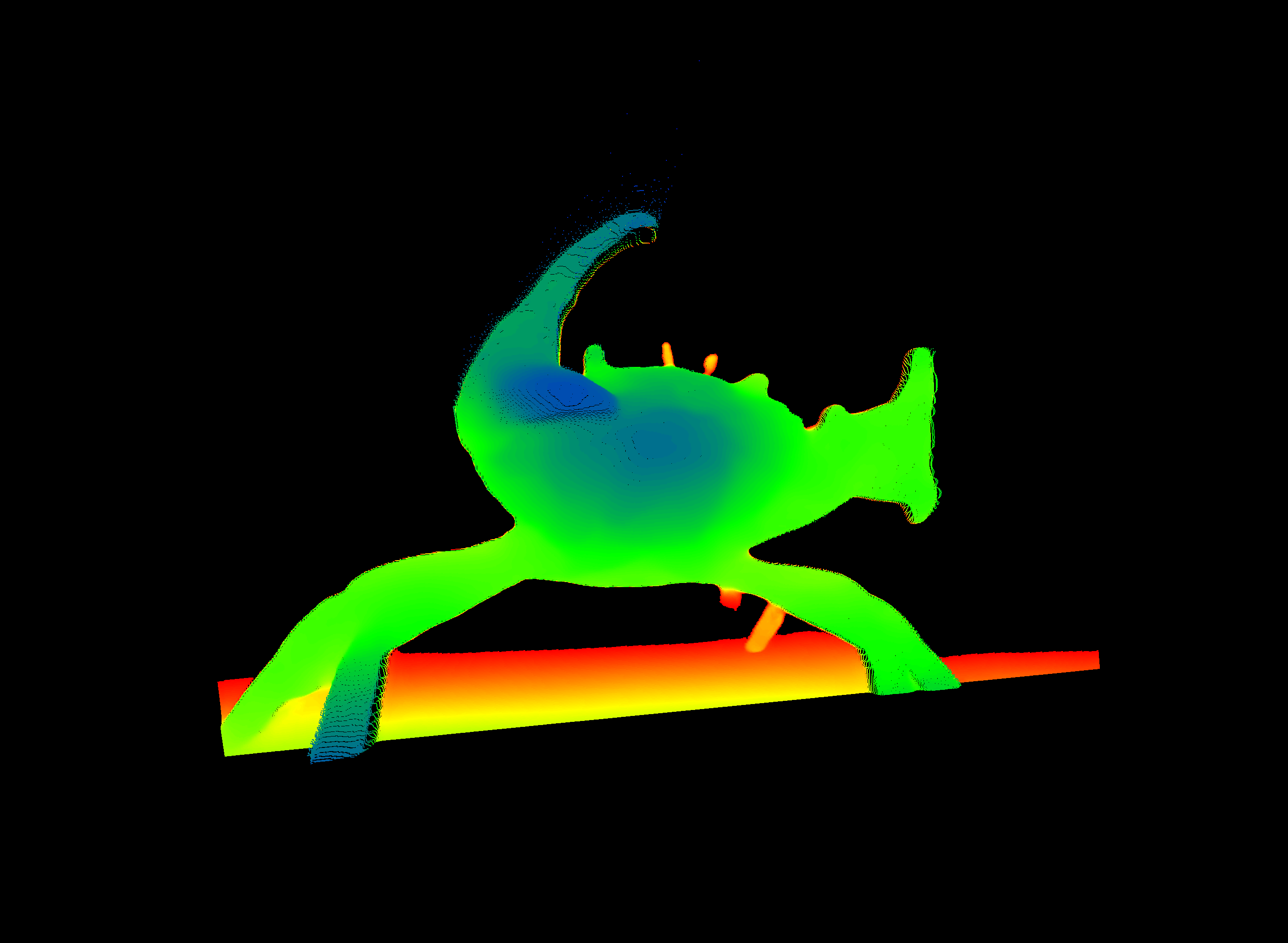
Apparently the human eye/brain cannot really comprehend the correctness of a depth image until its viewed in 3D. So I need to go on a deeper research for a newer and/or better model.

Getting something from ByteDance’s Video Depth Anything

#

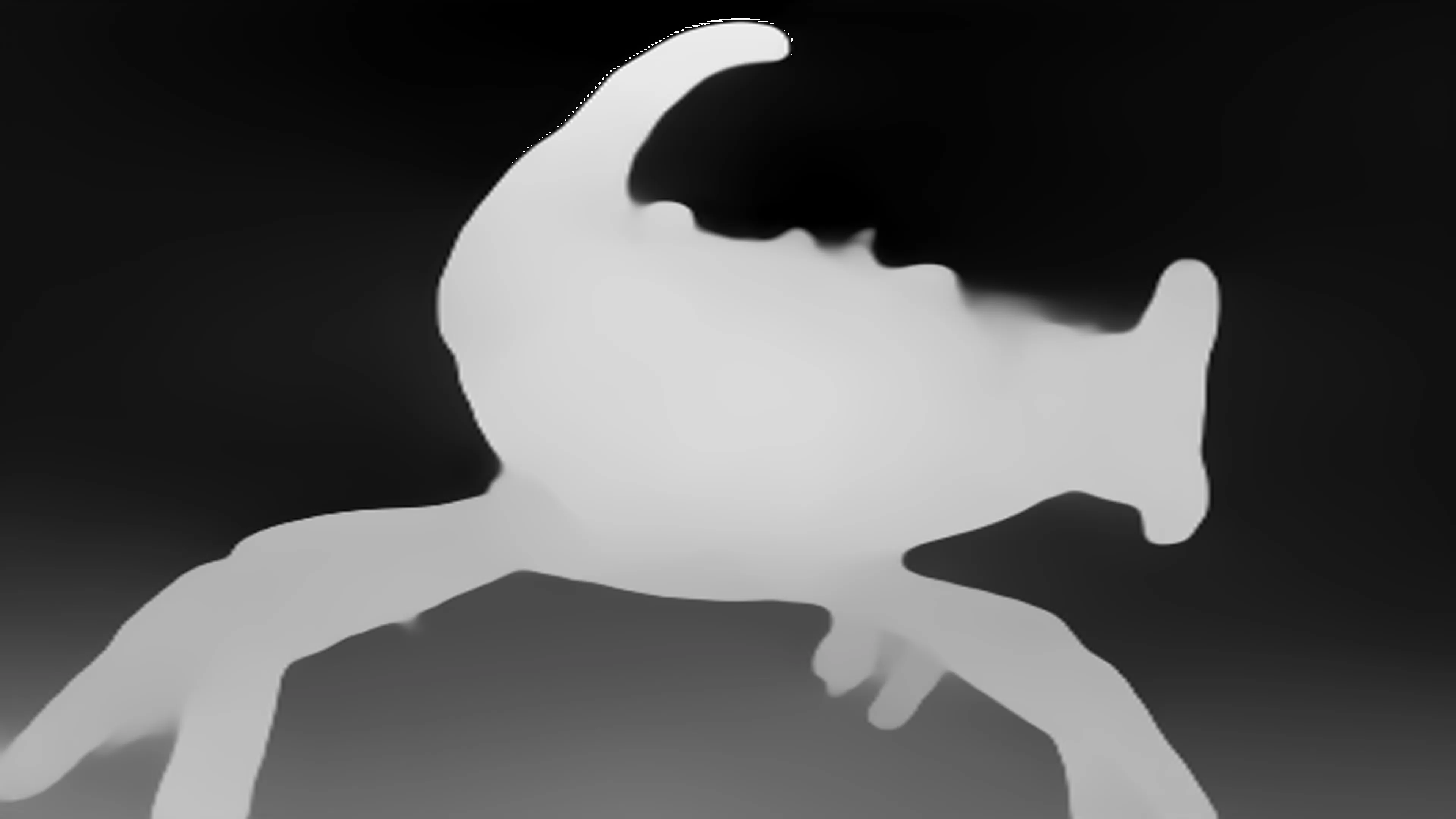
I quickly found another model, where I was not really sure i I could run this on my hardware. It is the Depth Anything V2 model from ByteDance, which I was able to test online on huggingface. The output of that tested frame can be seen in the following figure.

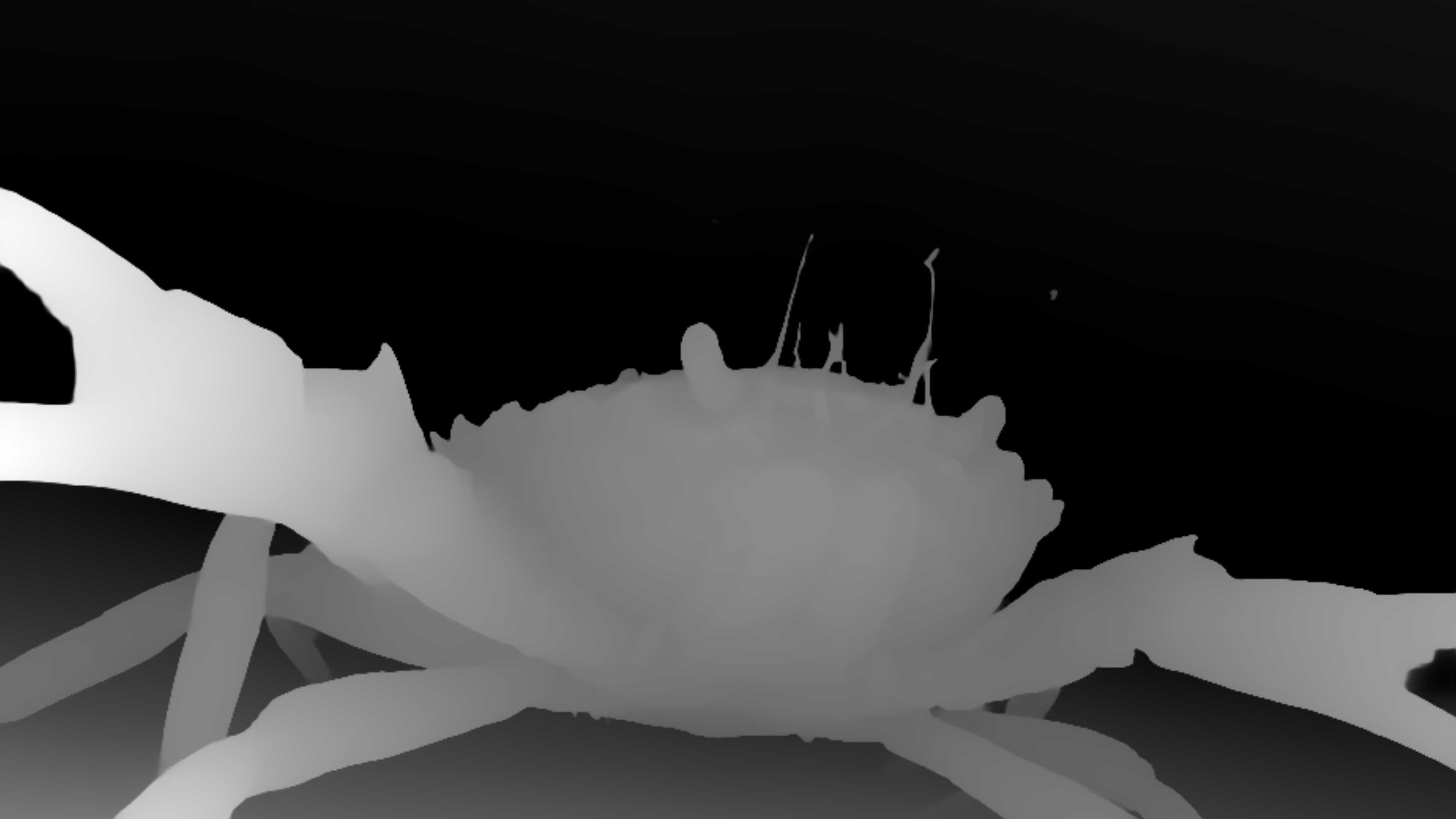
The new model does not only cleanly detect the outline of the eyes and the claws, but also the anterolateral teeth and the algae-covered antennae of the crab are resolved now.

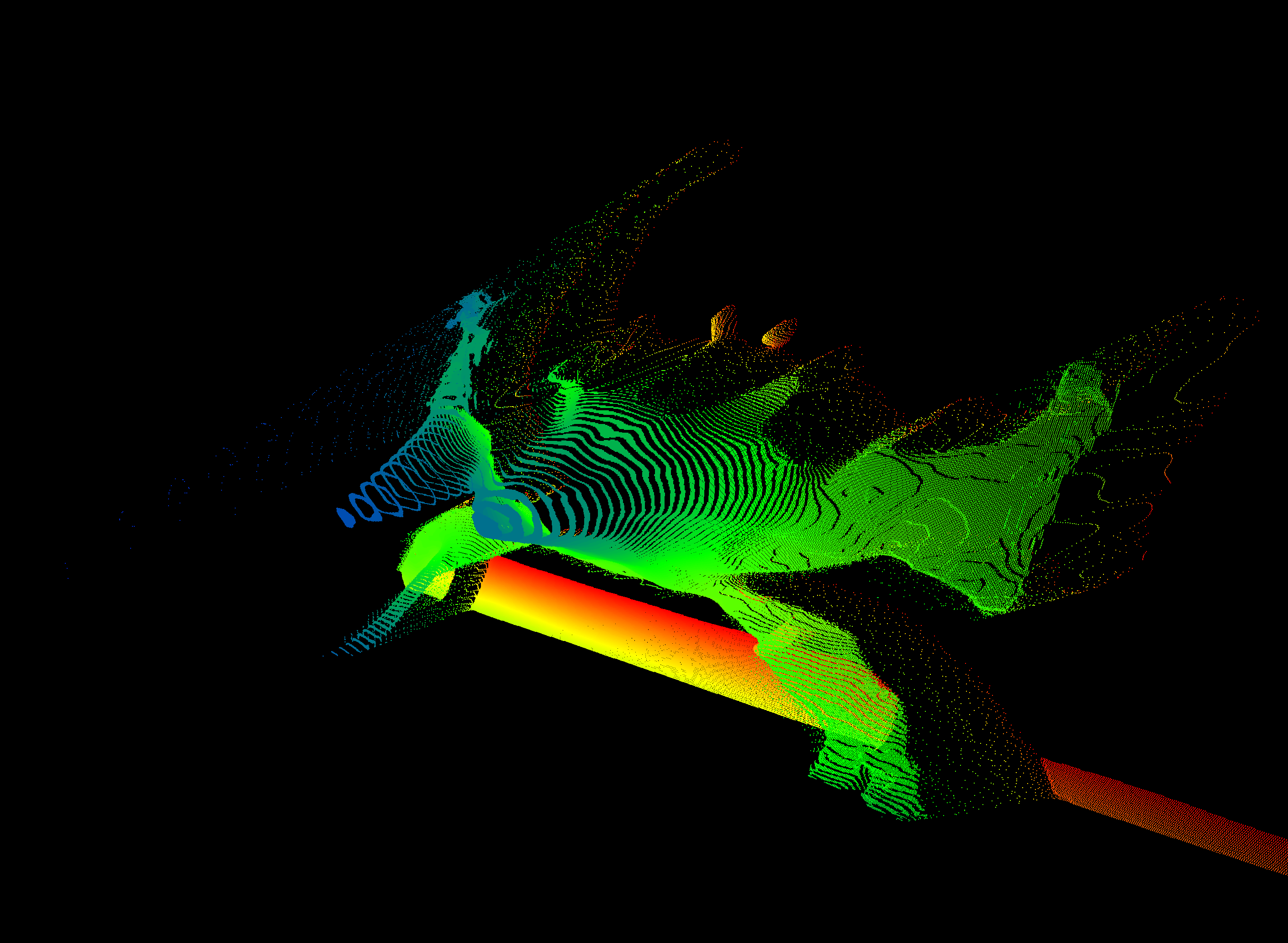
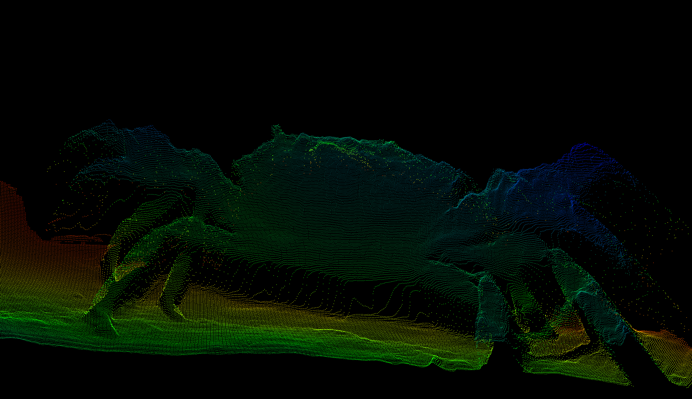
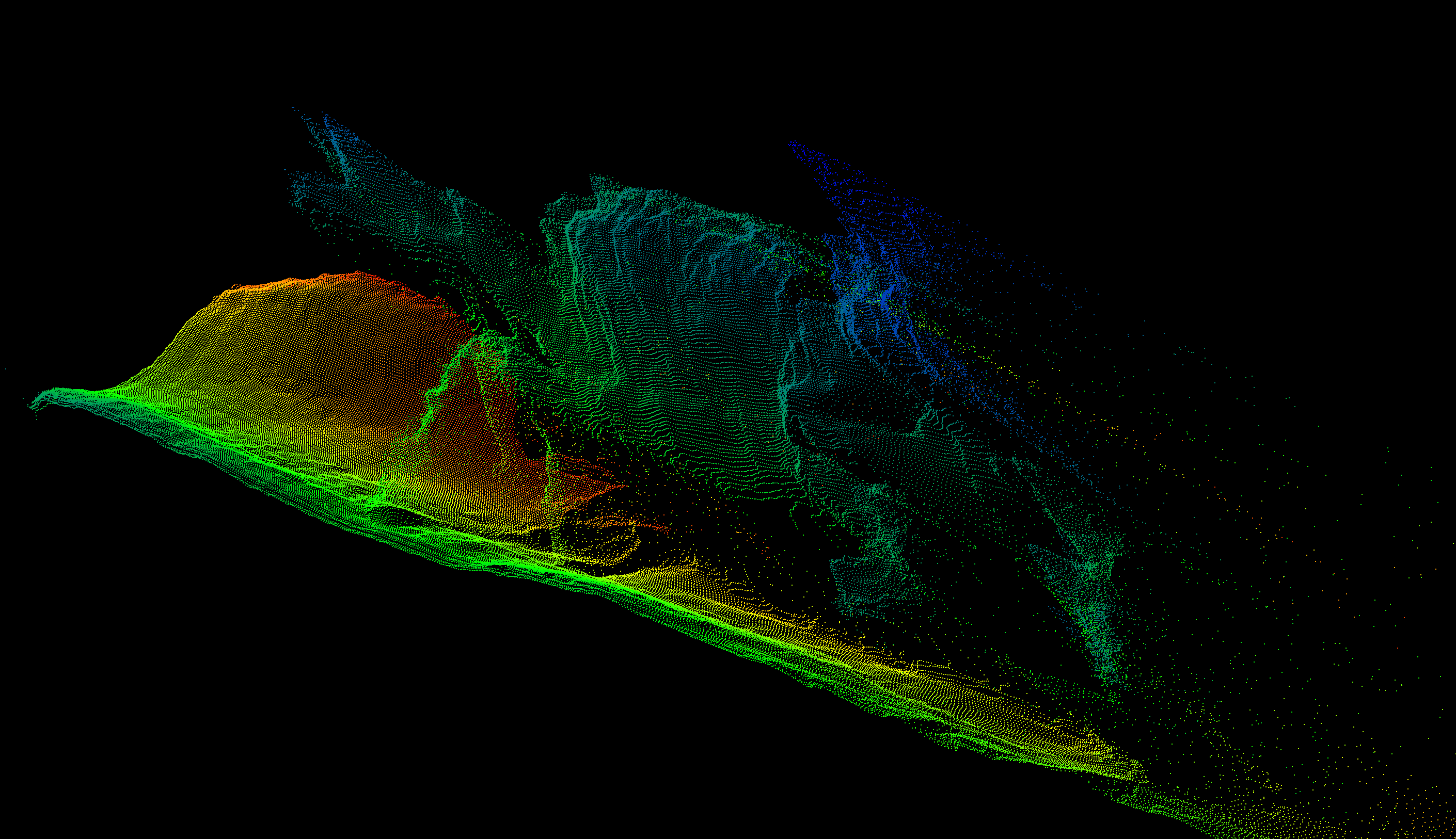
This is promising, but an issue, that I have ran into with the other will be an issue here too - temporal consistency. However there is a video variant of the model called Video Depth Anything (surprise). It is actually based on the second version of the still image model. Looking at a point cloud, projected from a still image, we have a much better depth estimation. It is still not perfect and breaking apart in certain places, but that is fine for doing some glitchy Blender art.

The Setup instructions are overall concise, but i needed to try some different Python versions until I found out that Python 3.11 seems to be the right version this works with.

Before continuing, I have scaled down and cropped the GoPro recording to reduce the need in computing power using ffmpeg. I used this step to simultaneously flip the video right-side-up.

ffmpeg -i GoPro.mp4 -vf "rotate=PI,scale=-1:720" -ss 10 -to 20 -c:a copy cropped_GoPro.mp4

After activating the venv, the first step is to get the weights for the model. This is done by bash get_weights.sh. There are essentially three models small, base and large. Naturally I want to archive best quality so I tried vitl (large) first and ran straight into memory limits on the 12G of my RTX4070 Super. To see if any of the models had any chance of running, I jumped to the smallest model, which worked but wasn’t very good looking. In the end, the base model (vitb; it is calles base but is actually more like the middle ground between small and large) was the one I will be using from here on. Adding the --metric flag will result in the export of a .ply sequence instead of a depth video. This is nice, as I want to use a sequence of .ply files anyways.

python3 run.py --input_video /home/.../cropped_GoPro.mp4 --output_dir ./outputs --encoder vitl
# Running into memory constraints

python3 run.py --input_video /home/.../cropped_GoPro.mp4 --output_dir ./outputs --encoder vits
# Looks a bit less good, than the initial test

python3 run.py --input_video /home/.../cropped_GoPro.mp4 --output_dir ./outputs --encoder vitb
# This seems to be a working middle ground

python3 run.py --input_video /home/.../cropped_GoPro.mp4 --output_dir ./outputs --encoder vitb --metric
# This is What is beeing used in the end

While Python 3.11 worked well, the requirements.txt of that project threw a lot of errors, to the point where I just installed the dependencies manually.

Blender magic

#

The rest of the pipeline happens in Blender (apart from merging the rendered result into a video file in the very end, which is done by ffmpeg; this could also be rendered as a video by Blender directly. However I wanted to try out a few options regarding formats and bitrate for using it as a background). First we need to import and then we need to style the point cloud data.

Import

#

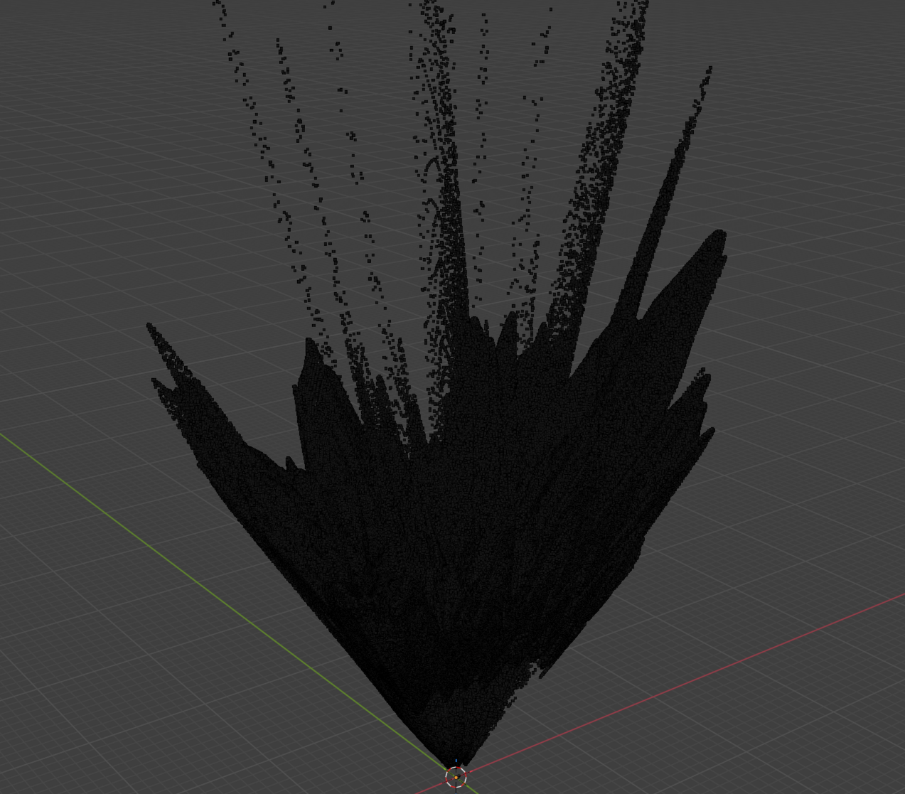
Ok so we got point clouds now … cool, finally! However there is still a bit to do. The sequence needs to be loaded into blender in a way, where it can be accessed by the geometry nodes, the geometry and shading node setups needs to be made and applied. And while blender supports the import of single .ply files, we can just import the whole time series via a script in the scripting tab of Blender.

import bpy
import struct
import os

# User settings
folder_path = "/x/y/z/ply_seq/"
start_frame = 1  # Which Blender frame to start the animation
point_size = 0.0005  # Size of points; cyn be changed in 

# Helper function to read binary PLY vertices
def read_binary_ply_vertices(filepath):
    with open(filepath, "rb") as f:
        line = f.readline()
        if not line.startswith(b"ply"):
            raise ValueError("Not a PLY file")
        
        vertex_count = 0
        while True:
            line = f.readline().strip()
            if line.startswith(b"element vertex"):
                vertex_count = int(line.split()[2])
            elif line.startswith(b"end_header"):
                break
        
        vertices = []
        for _ in range(vertex_count):
            # Unpack spacial data, ignore rgb
            data = f.read(27)  # 3 doubles * 8 bytes
            x, y, z,_ ,_ ,_ = struct.unpack("<dddBBB", data)
            vertices.append((x, y, z))
        
        return vertices

# Load all PLY files
ply_files = sorted([f for f in os.listdir(folder_path) if f.endswith(".ply")])
all_verts = []
frame_numbers = []

print(f"Loading {len(ply_files)} PLY files...")
for i, ply_file in enumerate(ply_files):
    filepath = os.path.join(folder_path, ply_file)
    verts = read_binary_ply_vertices(filepath)
    all_verts.extend(verts)
    frame_numbers.extend([start_frame + i] * len(verts))
    print(f"  Loaded {ply_file}: {len(verts)} points (frame {start_frame + i})")

print(f"Total points: {len(all_verts)}")

# Create single mesh & convert to point cloud
mesh = bpy.data.meshes.new("PointCloud_Mesh")
obj = bpy.data.objects.new("PointCloud_Animation", mesh)
mesh.from_pydata(all_verts, [], [])
mesh.update()
bpy.context.collection.objects.link(obj)

# Convert to point cloud
bpy.context.view_layer.objects.active = obj
obj.select_set(True)
bpy.ops.object.convert(target='POINTCLOUD')
obj.select_set(False)

# Add frame_nr attribute - This is needed so the points can be hidden on all other frames
frame_attr = obj.data.attributes.new(name='frame_nr', type='INT', domain='POINT')
for i, point in enumerate(frame_attr.data):
    point.value = frame_numbers[i]

# Set point radius
if 'radius' not in obj.data.attributes:
    radius_attr = obj.data.attributes.new(name='radius', type='FLOAT', domain='POINT')
else:
    radius_attr = obj.data.attributes['radius']

for point in radius_attr.data:
    point.value = point_size

print(f"Done! Created single point cloud with {len(all_verts)} points across {len(ply_files)} frames")

The script will scan the supplied directory for ply files, sort them by name and import them in that order into a single point cloud object in Blender.

On import the script appends the frame number to every point, so we can use that value later for selecting a subset of the cloud per frame. While it is possible to import each .ply file as a separate object and simply hide/show objects per frame via script, that approach has several drawbacks:

• We cannot easily move the whole object as one (we would need to do some parenting.)
• As the reveal logic is handled in geometry nodes later, we are much more flexible for changing things around later. For example, we can do speedups/slowdowns by repeating cloud frames or skipping some. This would be basically impossible if there was a bunch of single objects per frame with it being displayed on a single a scripted frame. One would need to change all timings for every consecutive frame manually
  • Indirectly this would also allow for some more effects in the time domain, e.g. a ghosting effect
• The geometry and shader node setup only needs to be applied to one object

Styling and Animation

#

Before applying a shader, we need a bit more overview. Thats why I have created a geometry node setup.

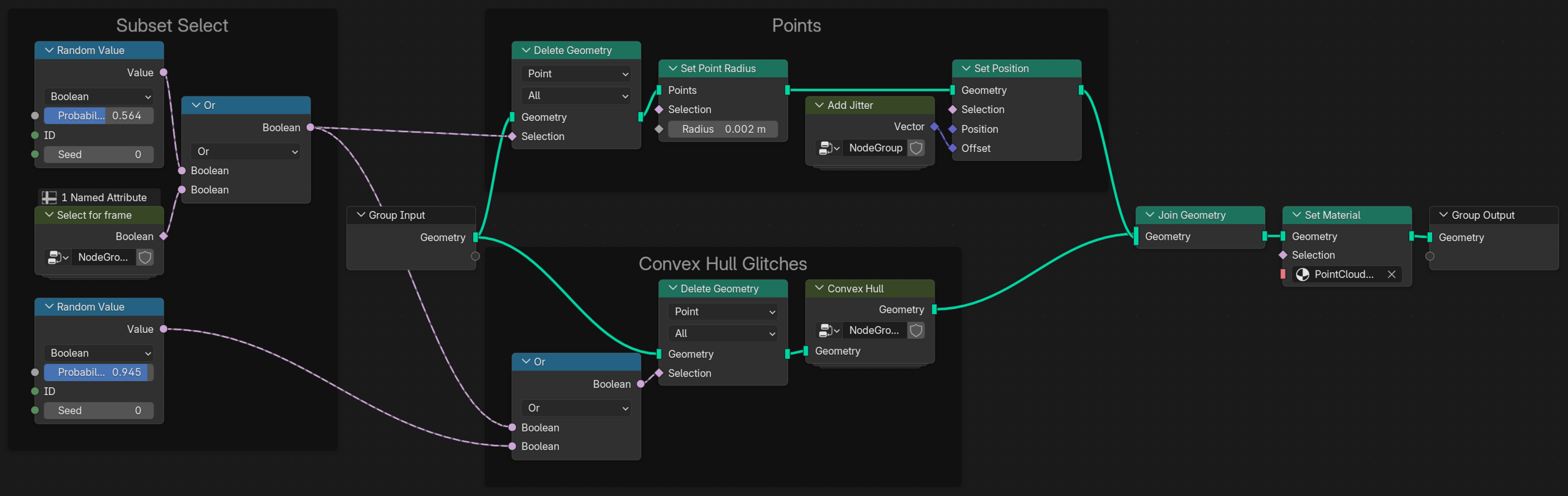
The nodes are basically sectioned into three categories (apart from the input output sections):

• Subset Select
  • This is where the full point cloud is reduced to a useful subset via the frame number and some random subsampling to hide the raster characteristic of the data
• Points
  • This is where the points can get a new radius (if the one on import was off) and a little jitter to make the appearance more organic.
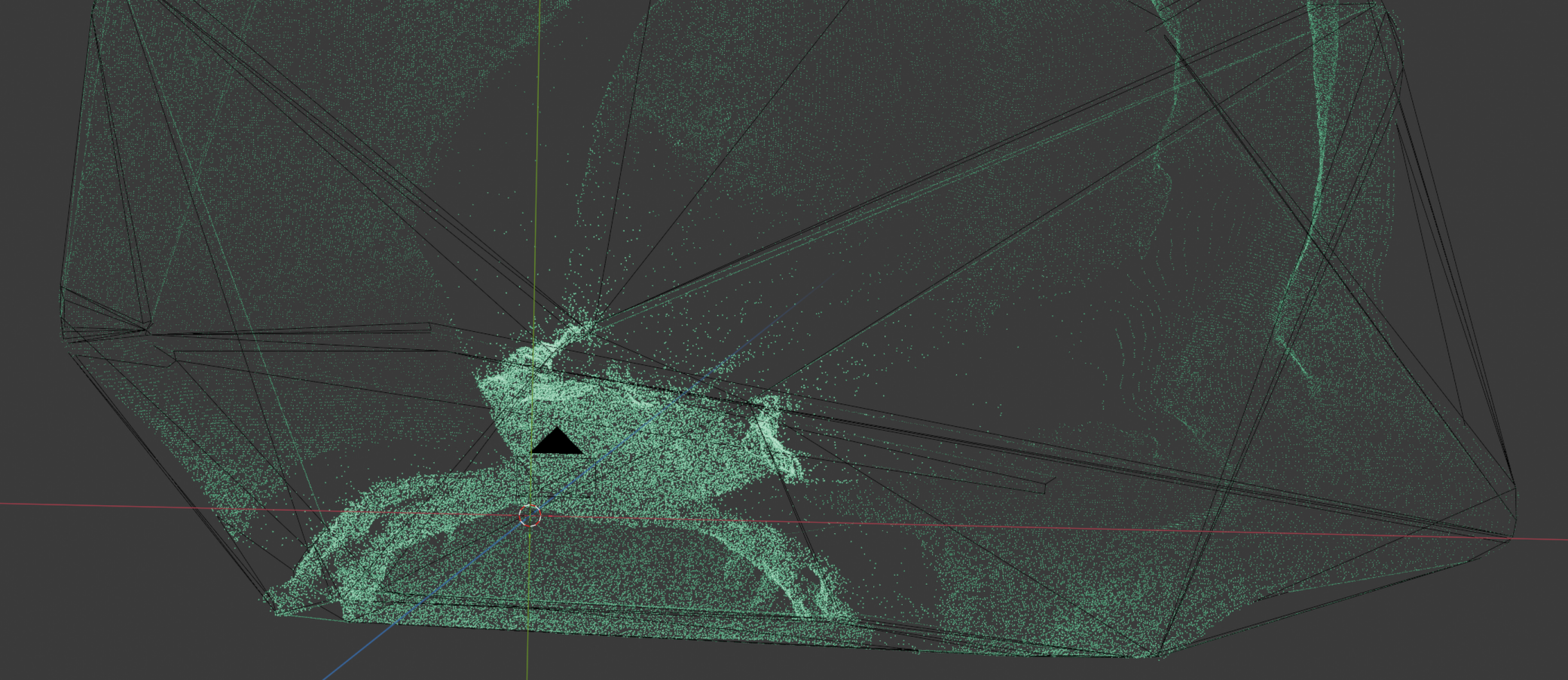
• Convex Hull Glitches
  • This a section that adds an additional layer of visual interest by utilizing the convex hull node

Select for frame

#

The frame selection happens by comparing the scene frame number with the point cloud number and inverting that selection to create a binary mask for the Delete Geometry node.

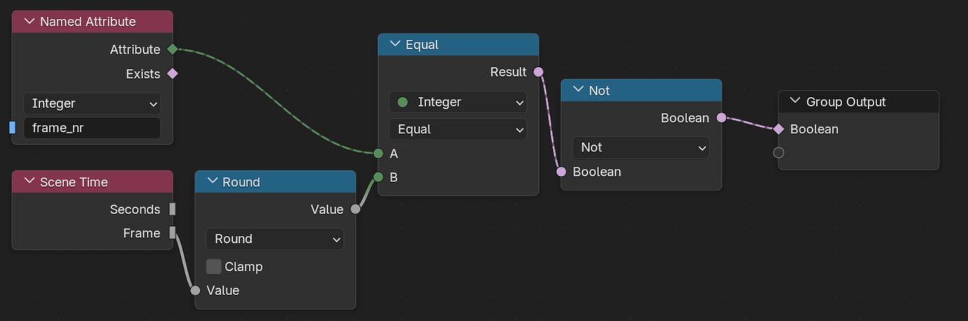
In the overview, we can see, that this is combined with a Random value via an Or to further reduce the number of points more than just to the single frame. This helps hiding the regular pixel grid from the depth image raster.

Convex Hull

#

Goal of this effect was to create an effect, where random points of the point cloud connect via a line each frame to get a little bit more interesting image.

Before the convex hull effect the geometry gets reduced once more to ‘shrink’ the effect into the remaining point cloud. Statistically, the points that will be used for that convex hull node span a smaller volume and are therefore ‘shrunken inside’ the previously selected cloud.

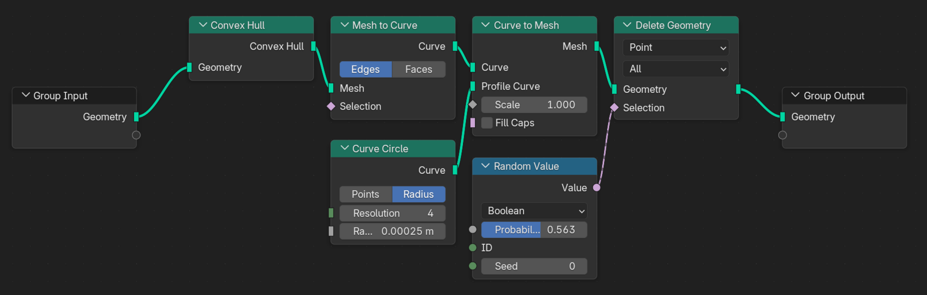
Initially, the convex hull is created, which results in a mesh. That mesh is converted int a curve, so a small circle can be extruded among the edges of the convex hull. The solid body of the convex hull has now gone to a wireframe with a thickness to all ‘wires’. The effect looks whacky, when all lines are left in. Therefore a random amount of that geometry is deleted again.

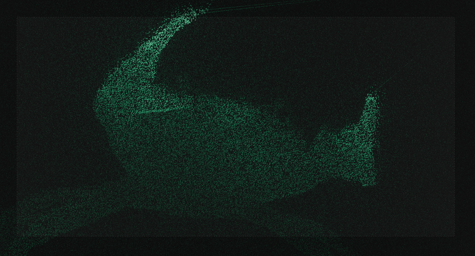
Shading

#

The shading is very simple. It is just a simple emission shader with the strength tuned to a value that looks good.

Volumetric Fog

#

To add some depth I added some volumetric fog effect via the Volume scatter shader applied to a large cube. That effect does look weird from far away.

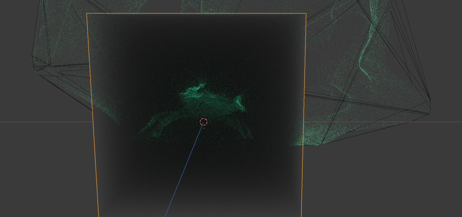
The effect works well, when viewd through an animated camera that follows the crab a bit.

Finalization

#

The only thing remaining is to add some glare in the blender compositing, render the sequence via cycles and then merging the sequence:

ffmpeg -framerate 15 -i %04d.png -c:v h264_nvenc -b:v 200M output.mkv

I am quite satisfied with this result, considering there was no depth information in my GoPro clip